This first tutorial will guide you through the process of setting up a new application using the DiFfRG. This first program will simply solve a hydrodynamic equation unrelated to fRG, but introduce the basic structure of a typical DiFfRG application.

You can find the full code as described here also in Tutorials/tut1.

File structure

We will start by creating a new directory in the Applications directory just below the DiFfRG top directory. This directory will contain all the files necessary for the simulation.

$ cd Applications
$ mkdir tut1
$ cd tut1
$ touch CMakeLists.txt
$ touch tut1.cc
$ touch model.hh
$ touch parameters.json

The CMakeLists.txt file is used to tell CMake how to build the project.
The tut1.cc file contains the main function of the simulation and the most general structure of the simulation.
In the model.hh file we will define the numerical model, i.e. the set of differential equations that we want to solve.
The parameters.json file will contain the parameters for the simulation.

CMake setup

The CMakeLists.txt file is the first thing we need to set up. CMake is a powerful build system which automates complex setup of dependencies and structure of C++ programs. For a deeper understanding, please consult the documentation and see the DiFfRG build system setup in DiFfRG/cmake/setup_build_system.cmake.

In our case, we need to tell CMake about our new simulation and about the DiFfRG library. In practice, our CMakeLists.txt file looks as in the following:

cmake_minimum_required(VERSION 3.26.4)
 
project(tut1)

In the above, we first request a minimum version of CMake and then declare our project.

find_package(DiFfRG REQUIRED HINTS /opt/DiFfRG)

Afterwards, we request CMake to find the DiFfRG package. We set the default install path here, which is /opt/DiFfRG, but depending on where you installed DiFfRG, you will have to change this.

add_executable(tut1 tut1.cc)

setup_application(tut1)

Finally, we register an executable with CMake (called tut1) and use the setup_application function, which is a part of DiFfRG. It sets up all dependencies necessary for a DiFfRG-application, sets header paths and links it against the DiFfRG library.

With this set up, we can immediately create our build directory and test the build system. To that end, create a new directory and enter it,

$ mkdir build

$ cd build

Then, invoke cmake,

$ cmake -DCMAKE_BUILD_TYPE=Release -DCMAKE_CXX_FLAGS='-O3 -march=native -ffast-math -fno-finite-math-only' ..

Here, we tell CMake to create an optimized "Release" build and propagate some further optimization flags to the compiler. The last argument to the cmake command, .., tells it where the source files can be found. In this case, it finds the CMakeLists.txt we just created in the parent directory and uses it to set up the build system.

At this point you could already invoke the build system by running

$ make -j8

which will build the whole project using 8 cores. However, doing this will at this stage only lead to a linker error, as the tut1.cc file does not contain anything yet. In particular, the program lacks an entry point, i.e. a main function.

tut1.cc

Now we are ready to set up the main structure of the program in tut1.cc.

#include <DiFfRG/common/configuration_helper.hh>
#include <DiFfRG/common/utils.hh>
#include <DiFfRG/discretization/discretization.hh>
#include <DiFfRG/timestepping/timestepping.hh>
 
#include "model.hh"
 
using namespace DiFfRG;
 
int main(int argc, char *argv[])
{

The includes in the first few rows are parts of the DiFfRG and we will use them in a moment to set up the simulation. Next, we include the model.hh file, where we will set up the actual system of equations to solve.

All relevant classes and functions are in the DiFfRG master namespace, so for convenience we just import all symbols from this namespace into our code by using namespace DiFfRG;.

The actual program logic starts with the entry point, the main function. The first thing to do in the main function is to read the parameter file parameters.json we created earlier:

// get all needed parameters and parse from the CLI
ConfigurationHelper config_helper(argc, argv);
const auto json = config_helper.get_json();

The ConfigurationHelper class automatically chooses the correct parameter file; if the executable is invoked with the -p parameter, i.e. ./tut1 -p parameters.json, the argument of -p is chosen as the parameter file. Otherwise, ConfigurationHelper will try to open a file called parameters.json in the current working directory. The parameters have to be specified in the JSON format.

In order for this class to parse the flags and arguments passed from the command line, we need to construct the object with the argc, argv parameters, which hold this information. Afterwards, we load the entire parameter structure into the json variable, which has the same structure as the original json file.

After setting up the configuration, we choose the algorithms used in our simulation. To do so, we make some convenient type aliases with the chosen class types:

// Choices for types
using Model = Tut1;
constexpr uint dim = Model::dim;
using Discretization = CG::Discretization<Model::Components, double, RectangularMesh<dim>>;
using VectorType = typename Discretization::VectorType;
using SparseMatrixType = typename Discretization::SparseMatrixType;
using Assembler = CG::Assembler<Discretization, Model>;
using TimeStepper = TimeStepperSUNDIALS_IDA<VectorType, SparseMatrixType, dim, UMFPack>;

After making an alias for the numerical model, which we will specify in a moment, we choose a spatial (field space) dimension, which is here simply taken from the Model.

The Discretization gives a prescription to discretize the field space. Here, we choose the CG, i.e. Continuous Galerkin discretization and accordingly a fitting Assembler. The assembler, as the name implies, assembles the system of equations to be solved. In practice, the differential equation you specify in the Model is discretized by the Assembler using the Discretization and brought into the form of a time-dependent, nonlinear ODE (ordinary differential equation)

\[ F(\partial_t v_i, v_i) = 0\,, \]

where $v_i$ are the components of the discretization. The Assembler is directly invoked by the TimeStepper which requests the construction of the above equation at every (RG) time step and evolves the system according to it. If you are unfamiliar with FEM methods, it would be recommended to at least understand the basics of it.

Next, we choose the SUNDIALS_IDA timestepper, which is the most performant choice for FEM setups with spontaneous symmetry breaking. IDA is a differential-algebraic solver, i.e. it solves both equations dependent on time, as above,

\[ F(\partial_t v_i, v_i) = 0\,, \]

but also stationary (secondary) equations without explicit dependence on time derivatives,

\[ G(v_i) = 0\,. \]

We will show the utility of this in a later tutorial. Note that the TimeStepper takes an additional argument, where we can choose the linear solver. The direct solver UMFPack is a simple but good choice, as it solves any linear system exactly. However, with large systems, e.g. in $d\geq2$, GMRES or another iterative solver is usually much faster and thus preferred.

// Define the objects needed to run the simulation
Model model(json);
RectangularMesh<dim> mesh(json);
Discretization discretization(mesh, json);
Assembler assembler(discretization, model, json);
TimeStepper time_stepper(json, &assembler);

We now use the types we defined above to construct objects of all the classes described above.

With everything prepared, we are now ready to set up and run the equation system. To do so, we create an initial condition on the discretization (i.e. FEM space) we set up before,

// Set up the initial condition
FE::FlowingVariables initial_condition(discretization);
initial_condition.interpolate(model);

and use it to run the time-stepper from RG-time 0 to the final RG-time, which we infer from the parameter file:

// Now we start the timestepping
Timer timer;
try {
  time_stepper.run(&initial_condition, 0., json.get_double("/timestepping/final_time"));
} catch (std::exception &e) {
  spdlog::get("log")->error("Simulation finished with exception {}", e.what());
  return -1;
}
auto time = timer.wall_time();

Note here, that RG-time is defined on the level of the code as positive, i.e.

\[ t_+ = \ln \Lambda / k \]

whereas the usual convention is

\[ t_- = \ln k / \Lambda \]

Furthermore, we recorded the time the simulation took using the dealii::Timer class.

We finish the program by printing a bit of information to the log file, in particular the performance and utilization of the Assembler.

  // We print a bit of exit information.
  assembler.log("log");
  spdlog::get("log")->info("Simulation finished after " + time_format(time));
  return 0;
}

model.hh

Now we need to specify the equation system to solve. For this example, we will just implement Burgers' equation, which is not fRG-related but a simple hydrodynamic equation given by

\[ \partial_t u(x,t) + \frac12 \partial_x u(x,t)^2 = 0 \]

First things first, we set a few things up before we get to the equation system:

#pragma once
 
#include <DiFfRG/model/model.hh>
 
using namespace DiFfRG;
 
struct Parameters {
  Parameters(const JSONValue &value)
  {
    try {
      a = value.get_double("/physical/a");
      b = value.get_double("/physical/b");
      c = value.get_double("/physical/c");
      d = value.get_double("/physical/d");
    } catch (std::exception &e) {
      std::cout << "Error in reading parameters: " << e.what() << std::endl;
    }
  }
  double a, b, c, d;
};

Although not necessary in this case, the #pragma once compiler directive ensures that the header file is not included multiple times (similar to the use of include guards), which would lead to compiler errors. The DiFfRG/model/model.hh header contains basic predefines necessary for the setup of a numerical model. Again, we import all symbols from the DiFfRG namespace.

Afterwards, we create a struct to hold parameters we read once from the JSON variable. We call these a,b,c,d and will use them to construct the initial condition for the differential equation, i.e. $u(x,0)$.

With this in place, let's set the equation system structure up:

using FEFunctionDesc = FEFunctionDescriptor<Scalar<"u">>;
using Components = ComponentDescriptor<FEFunctionDesc>;
constexpr auto idxf = FEFunctionDesc{};

Our system is very small, consisting only of a single equation. With large fRG simulations this can grow however extremely large, using momentum grids of variables and large vertex expansions. Thus, DiFfRG provides a mechanism of describing these systems and smartly indexing the numerical degrees of freedom. Here, we use a descriptor to tell the library how many and what kinds of functions we have. We use one function which lives on a FEM discretization and thus use the FEFunctionDescriptor with one Scalar which we call "u" as in the above equation.

If we had two variables, e.g. another one called $v$, we would declare this as FEFunctionDescriptor<Scalar<"u">, Scalar<"v">>;. We will treat the declaration of larger systems in a later tutorial in-detail.

The ComponentDescriptor type packs the FEFunctionDescriptor together with other parts of the equation system; here, we only have a FE function and thus do not provide more template parameters. Creating a compile-time constant (constexpr) object of the descriptor is useful for easier access to the indices, which we will use below.

 
class Tut1 : public def::AbstractModel<Tut1, Components>,
             public def::fRG,                  // this handles the fRG time
             public def::FlowBoundaries<Tut1>, // use Inflow/Outflow boundaries
             public def::AD<Tut1>              // define all jacobians per AD
{

Now we define the actual numerical model. We need to derive the class from def::AbstractModel, which defines all necessary methods so our numerical model can be used by the Assembler. Here, we also communicate the structure of our equation system through the Components type we declared earlier. Furthermore, we derive from a few more classes:

def::fRG provides a method where $t$ is automatically communicated to the model and the RG-scale $k$ is computed from it. Furthermore, it defines the variables t and k which can be directly used in the code.
def::FlowBoundaries is necessary to close the FEM system, as the boundary conditions at $x=0$ and $x = x_\textrm{max}$ need to be specified. def::FlowBoundaries sets up inflow/outflow boundary conditions.
def::AD creates methods for the automatic evaluation of jacobians of our system, i.e.
\[ \frac{\partial (\partial_t u - \frac12 \partial_x u^2)}{\partial u}\,\qquad\text{and}\qquad \frac{\partial (\partial_t u - \frac12 \partial_x u^2)}{\partial (\partial_t u)}\,. \]
This is achieved by the use of automatic differentiation, using the autodiff library. This is also the reason why we must template and not use explicit types in the methods of the numerical model, as will be seen below.

private:
  const Parameters prm;
 
public:
  static constexpr uint dim = 1;
 
  Tut1(const JSONValue &json) : def::fRG(json.get_double("/physical/Lambda")), prm(json) {}

Here, we have only written the constructor, communicated $\Lambda$ to the def::fRG base class and created a Parameters object.

template <typename Vector> void initial_condition(const Point<dim> &x, Vector &values) const
{
  const auto x = x[0];
  values[idxf("u")] = prm.a + prm.b * powr<1>(x) + prm.c * powr<2>(x) + prm.d * powr<3>(x);
}

The initial_condition method is invoked by the initial_condition.interpolate(model) call from above. We use the parameters a,b,c,d to set up a polynomial initial condition. Here, we also use the indexing provided by the FEFunctionDescriptor class, to retrieve the position of "u" within the array of FE functions. In this case, it is of course trivial, as idxf("u") always evaluates to 0. Note however, that the lookup is done statically at compile time and is thus much faster than dynamic lookup, such as with a std::map.

  template <typename NT, typename Solution> void flux(std::array<Tensor<1, dim, NT>, Components::count_fe_functions(0)> &F_i, const Point<dim> &/*x*/, const Solution &sol) const
  {
    const auto &fe_functions = get<"fe_functions">(sol);
 
    const auto u = fe_functions[idxf("u")];
 
    F_i[idxf("u")][0] = 0.5 * powr<2>(u);
  }
};

The flux method implements the actual equation. If we don't specify anything else, the Assembler will construct the equation

\[ \partial_t u + \partial_x (F_i(u)) = 0 \]

so that our choice of $F_i(u) = - \frac12 u^2$ exactly implements Burgers' equation.

parameters.json

The parameter file contains usually user-defined quantities in a "physical" subsection and further paramters for the backend:

{
  "physical": {
    "Lambda" : 1.0,
    "a" : 0.0,
    "b" : 1.0,
    "c" : 0.0,
    "d" : 0.0
  },

These sections are just the parameters we also use in the numerical model, i.e. user-space parmeters.

"discretization": {
  "fe_order": 3,
  "threads": 8,
  "batch_size": 64,
  "overintegration": 0,
  "output_subdivisions": 2,
 
  "EoM_abs_tol": 1e-10,
  "EoM_max_iter": 100,
 
  "grid": {
    "x_grid": "0:1e-2:1",
    "y_grid": "0:0.1:1",
    "z_grid": "0:0.1:1",
    "refine": 0
  },

The discretization section configures the FEM setup of our simulation:

fe_order sets the polynomial order of the local function space on the finite elements
threads sets the number of CPU threads used for assembly. Note, that other multithreading parts of DiFfRG, such as momentum integration, automatically use all available CPU threads and ignore this parameter.
batch_size the assembly threads get batches of batch_size which they sequentially process. Playing around with threads and batch_size may give a small performance boost, but keeping threads around the number of physical cores and batch_size around 32-64 should be sufficient for almost optimal performance.
overintegration can be used to increase the order of the quadratures used in assembly when constructing the weak form of the PDE. It is seldom necessary to increase beyond 0.
output_subdivisions gives the precision with which the grids in the output data are written. This goes exponentially, so don't choose it too high.
EoM_abs_tol sets the absolute precision within which a specified equation of motion is solved. DiFfRG can be instructed to solve the EoM at every timestep and perform additional computations at this point.
EoM_max_iter sets the number of bisections used in determining the position of the EoM.
x_grid this works in a python-like slice syntax and sets the used in a RectangularMesh. The parameter also supports locally different cell sizes: "0:1e-4:1e-2, 1e-2:1e-3:1" creates 100 cells between 0 and 1e-2, and 100 cells between 1e-2 and 1.
y_grid and z_grid work identically, but are only used in 2D / 3D simulations.
refine can be used to quickly increase the cell count by $2^\textrm{refine}$.
"adaptivity": {

"start_adapt_at": 0E0,

"adapt_dt": 1E-1,

"level": 0,

"refine_percent": 1E-1,

"coarsen_percent": 5E-2

}

},

The adaptivity section sets parameters for adaptive refinement of the discretization mesh. As we have not set this up in the numerical model, we will postpone the explanation of this section to a later tutorial.
"timestepping": {

"final_time": 10.0,

"output_dt": 1E-1,

"explicit": {

"dt": 1E-4,

"minimal_dt": 1E-6,

"maximal_dt": 1E-1,

"abs_tol": 0.0,

"rel_tol": 1E-3

},

"implicit": {

"dt": 1E-4,

"minimal_dt": 1E-6,

"maximal_dt": 1E-1,

"abs_tol": 1E-13,

"rel_tol": 1E-7

}

},

The timestepping section controls the behavior of the Timestepper class:
final_time sets the end-time of the simulation - this is actually not a required parameter, but one we use in our call to timestepper.run(...)
output_dt sets the intervals within which we write the solution to disk. Note, that the timesteppers do not necessarily step exactly onto output_dt intervals, but interpolate the solution to the output times.
The explicit and implicit sections control the behavior of explicit and implicit timesteppers respectively. The disctinction exists, because some timesteppers actually run part of the equation system explicitly and another implicitly. Usually, the FEM part is always implicit and further components of the expansion can be chosen to evolve explicitly.
- dt is the initial timestep for adaptive timesteppers and the fixed timestep for non-adaptive ones.
- minimal_dt and maximal_dt set the bounds for the timestep size - if an adpative stepper goes above or below, the step is adjusted to the bound, if the timestepper gets stuck below mminimal_dt, time evolution is aborted.
- abs_tol and rel_tol set absolute and relative error tolerance for the timestepping. While the FE parts of the system usually require a higher precision (< 1e-7 relative precision), especially in the presence of spontaneaous symmetry breaking, explicit tolerances can be chosen much more freely. For more information about timesteppers and their relationship with spontaneous symmetry breaking in fRG, see also this paper.

  "output": {
    "verbosity": 0,
    "folder": "./",
    "name": "output"
  }
}

The output section defines:

verbosity sets how much information is being written to console while running. If at 0, no information is written at all, whereas at 1 the system gives updates at every timestep.
folder sets the base folder where data is stored. This is useful to not clutter your current directory ("./") with output, or if you run a large amount of simulations.
name sets the beginning of all filenames of the output, i.e. in this case all files created by the simulation start with "output".

Running it

To run the simulation, first build it,

$ make

and then directly run it through

$ ./tut1 -p ../parameter.json -si /output/verbosity=1

We made use here of a mechanism to override the parameters of a simulation. The flag -p selects the parameter file to be used. By default it looks for a parameter.json in the current directory. One can use the flags -si to set an integer, -ss to set a string and -sd to set a double (floating-point) value, followed by the full path to the parameter and its value after an equality symbol.

After the simulation has run, which should take (depending on your computer) a few seconds, a few files have been created in the current folder, which you can look up by

$ ls -l

output.log contains logging information:
$ cat output.log

[2024/10/11] [23:01:31] [DiFfRG Application started]

[2024/10/11] [23:01:31] [FEM: Number of active cells: 100]

[2024/10/11] [23:01:31] [FEM: Number of degrees of freedom: 301]

[2024/10/11] [23:01:31] [FEM: Using 8 threads for assembly.]

[2024/10/11] [23:01:32] [CG Assembler:

Reinit: 4.36692ms (1)

Residual: 0.184398ms (3557)

Jacobian: 1.24521ms (17)

]

[2024/10/11] [23:01:32] [Simulation finished after 1s]
output.log.json contains a copy of the JSON parameters used.
output.pvd contains links to the FEM output data of the simulation and can be now visualized in Paraview.

After invoking $ paraview output.pvd, we open a new tab and choose line chart view:

Paraview interface

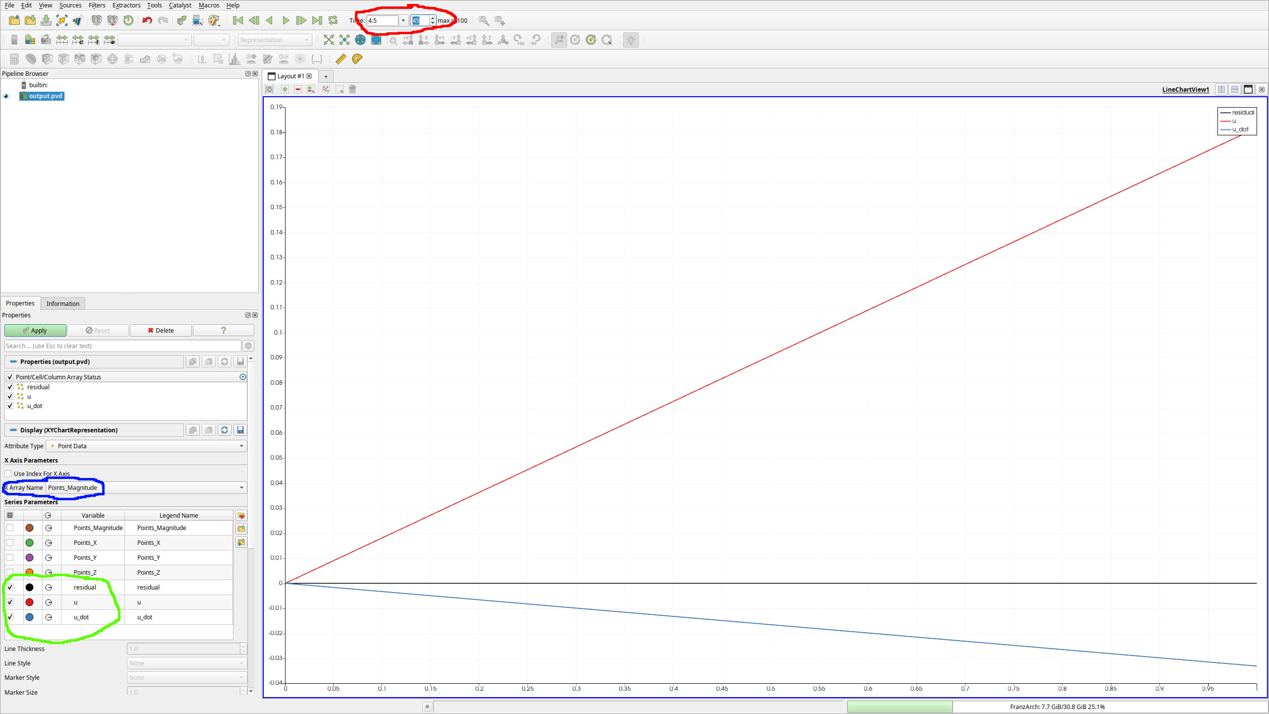
At the red marked field, one can change the currently displayed time of the FEM function.
The field marked in blue defines what the x-axis is. The default sets this to indices, but this does not work well in general and especially for irregularily spaced grids. Therefore, one would usually set this to Points_Magnitude for a 1D FEM simulation.
In the green marked part you see that we have the FE functions u, residual and u_dot which we can look at. u of course is just the solution to Burgers' equation, u_dot is its time derivative, and residual is the local error of the equation.

Feel free to play around also with the parameters a,b,c,d and other parts of the parameters in order to get acquainted with the basics of the framework.